Brittney Miller Math 5010

Even though Newton and Leibniz invented calculus independently from one another, they did have the similar approaches to problems. For example, Leibniz used a more geometric approach. He reasoned that if  where a  is a rectangle with sides  and ,can be thought of as the change in area when  is changed by  and  is changed by This is illustrated below. He then divided up the changed areas and compared them. So,  Here is where most people with even a basic mathematical background may scratch their heads; he reasoned that thesection was smaller than the infinitely small other rectangles so he justified just leaving it out based on his thought that it was so small, it would be okay to leave it out.(Boman, Rogers).

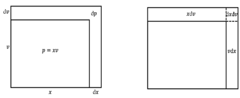
Thus, from Leibniz, we get the product rule as

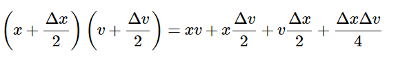
Meanwhile, in “The Principia”, Newton approach to the product rule comes from the incrementing and by and  as follows :

Then, he decremented  and  by the same amounts to get:

.

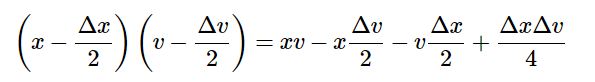Lastly, he subtracted the two equations and ended with . While this looks the same as the product rule we use today, there was a problem with the approach. This approach requires that the increments are 1⁄₂. Other numbers do not work.

Meanwhile, with Riemman sums, we can approximate the area under curves with simple geometry, similar to that of the Greeks. Riemman sums first divide the area under the curve into partitions. They use shapes of the same width to approximate the area of a finite curve. Typically rectangles, trapezoids, parabolas, or cubics are used. Similar to what the Greeks discovered 2,000 years before, the higher the number of partitions, the more accurate the approximation is. Within the use of different shapes, there are also different methods of using Riemman sums such as left rule (constructing the shape using the height of the point of the left of the partition), right rule (constructing the shape using the point of the right of the partition, midpoint rule (averaging the right and left points and using that as the height of the shape), upper rule (using the highest point in the partition), and lower rule (using the lowest point in the partition to construct the height on the shape). After the area is partitioned into one of the five rules, the area of each shape is taken and added up. For instance, if given a graph of y=x² where 1 ≤ x ≤ 5 we could approximate the area by using a right hand Riemann sum. If we use a partition number of 4, this would be evaluated by adding 4+9+16+25=54. By taking the integral, we see that 41.3 is the true value. Thus, the approximation is 12.7 off. If we were to increase the partitions to 20, the approximate would be 43.9 which would make the error 2.6. The following graphic illustrates this point by comparing the true value of the area to the different approximations using the different types of sums and a partition of 4 compared to 20.
Check our the applet below to explore Riemman Sums.